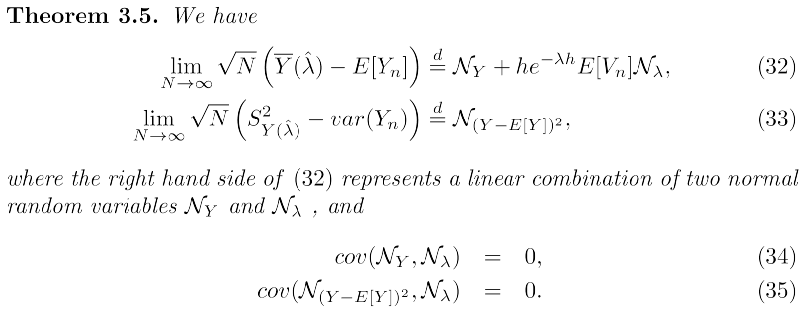
class: center, middle, inverse, title-slide # Moment estimators for parameters of Lévy-driven Ornstein-Uhlenbeck processes ### 吴燕丰， 江西财经大学 ### a joint work with 胡建强 and 杨翔宇 ### 2021-07-25 --- # Ornstein-Uhlenbeck (OU) process Stochastic Differential Equation (SDE): $$ dv(t) = -\lambda v(t)dt + dl(\lambda t) $$ where `\(l(t)\)` is a Lévy process (**B**ackground **D**riving **L**évy **P**rocess: **BDLP**), i.e., satisfying the following properties: 1. `\(l(0) = 0\)` almost surely; 2. Independence of increments; 3. Stationary increments. -- Examples of Lévy process: - Brownian motion - Poisson process, Compound Poisson Process - Gamma process, ... --- # A trajectory of an OU process .center[] ??? --- # Applications of OU process - stochastic volatility, Barndorff-Nelsen and Shephard model (**BNS** model) - membrane potential of a neuron - earthquake series - Levy-driven CARMA (Continuous ARMA, **A**uto**R**egressive **M**oving **A**verage) - **COVID19**: modelling the daily increment series? ??? - interest rate, Cox-Ingersoll-Ross model (**CIR**-model) --- # Literature Most previous works have been carried out for OU processes driven by special types of Lévy processes, such as: - **nonnegative Lévy processes** Jongbloed et al. (2005), Jongbloed and Van Der Meulen (2006), Zhang et al. (2006), Brockwell et al. (2007), Leonenko et al. (2013) - **compound Poisson processes** Zhang and Zhang (2010), Wu et al. (2019) - **α-stable Lévy processes** Hu and Long (2009), Zhang and Zhang (2013) - other types Long (2009), Masuda (2010), Taufer and Leonenko (2009), Valdivieso et al. (2009) --- # Literature OU processes driven by **general Lévy processes**: - Mai (2014), **MLE** for the drift parameter `\(\lambda\)` only - Spiliopoulos (2009), **Method of Moments** for all the parameters ### Our contributions - proposed a new MM estimation, related to Spiliopoulos (2009), with Smaller asymptotic variances - a Central Limit Theorem with an explicit Covariance Matrix - asymptotic variance `\(1-\rho^2\)` for the correlation estimator `\(\hat{\rho}\)`, same as that of the OLS estimator for a Gaussian AR(1) model .footnote[ Note: `\(\rho=e^{-\lambda h}\)` ] --- # SDE Solution and discrete samples $$ dv(t) = -\lambda v(t)dt + dl(\lambda t) $$ Integrated: $$ v(t) = e^{-\lambda t}\left(v(0)+ \int_{0}^te^{\lambda s}dl(\lambda s) \right) $$ Discretely Observed Samples $$ v_n \triangleq v(nh), n= 0,1,\cdots,N $$ Recursive equation $$ `\begin{equation*} v_n=e^{-\lambda h}v_{n-1} + \int_{(n-1)h}^{nh} e^{\lambda(s-nh)}dl(\lambda s) \end{equation*}` $$ --- # Method of Moments Define a new variable `$$y_n(\lambda) \triangleq v_n - e^{-\lambda h}v_{n-1}$$` ### Estimation of `\(\lambda\)` Autocovariance and autocorrelation of v(t): $$ `\begin{align*} \gamma(s) &= cov(v(t+s),v(t)) = e^{-\lambda s}var(v(t)),\\ \rho(s) &= corr(v(t+s),v(t)) = e^{-\lambda s}, \end{align*}` $$ Sample autocovariance and autocorrelation: $$ `\begin{eqnarray*} \hat{\gamma}_N(sh) &=& \frac{1}{N-s+1}\sum_{i=0}^{N-s}(V_{i+s}-\overline{V})(V_i-\overline{V}),\\ \hat{\rho}_N(sh) &=& \frac{\hat{\gamma}_N(sh)}{\hat{\gamma}_N(0h)}, \end{eqnarray*}` $$ --- ### Central Limit Theorem   --- # Estimation of the other parameters The first two (central) moments of `\(y_n(\lambda)\)` can be estimated by `\begin{eqnarray*} E[y_n(\lambda)] & \approx & \overline{Y}(\lambda) \triangleq \frac{1}{N}\sum_{n=1}^{N}Y_n(\lambda), \\ E[(y_n(\lambda)-E[y_n(\lambda)])^2] & \approx & S_{Y(\lambda)}^2 \triangleq \frac{1}{N}\sum_{n=1}^{N}(Y_n(\lambda)-\overline{Y}(\lambda))^2. \end{eqnarray*}` The higher moments of `\(y_n(\lambda)\)` can be estimated similarly if needed. --- ### Central Limit Theorem  --- ### Comparison: Smaller Asymptotic Variance  --- # Numerical Experiments .center[ <img width=500 src='images/table-1.png'> ] Table 1: A comparison between our method and MM-SP under different values of `\(λ\)` for OU process driven by a Lévy process composed of a Wiener processand a compound Poisson process --- class: middle, center Questions & Answers Thanks for Listening!